
Implementing the Modern LLM Stack: Grouped-Query Attention (Part 2)
Transitioning from Multi-head Attention to Grouped Query Attention, with KV Cache, GPU Trade-offs and the PyTorch implementation.

In this series of articles, we move beyond treating LLMs as black boxes and instead focus on understanding these design choices and then also implement these advancements in PyTorch.
This is Part 2 of the series where we dive deep into the Attention Mechanism, simplify complex topics like KV Cache, Multi-head attention, Grouped Query Attention, GPU Bottlenecks of LLM Inferencing, etc.
The Roadmap:
Part 2 (This Article): Efficient Attention – Implementing Grouped Query Attention (GQA) and integrating it with RoPE.
Part 3: Stability & Activation – Replacing LayerNorm/ReLU with RMSNorm and SwiGLU.
Part 4: Mixture of Experts – Building Mixture of Experts (MoE), including Top-k routers and load-balancing losses.
Part 5: Inferencing and Upcycling – Bringing it all together into a fully functioning, trainable model.
Part 6: Pre-training with various bells and whistles – Writing an optimised pre-training loop.
So let’s begin!
Quick Recap: Multi-Head Attention
Multi-Head Attention is the original attention mechanism introduced in Attention is All You Need (Vaswani et al., 2017). In MHA, each token’s embedding is linearly projected into multiple sets of Query (Q), Key (K), and Value (V) vectors. Each attention “head” uses its own Q, K, V to attend to other tokens, and the results from all heads are concatenated to form the output. This allows the model to focus on different aspects of token relationships in parallel.
If you are unfamiliar with attention, please refer to the following resources:
The Illustrated Transformer and The Illustrated GPT-2 by Jay Alammar. This post offers an amazing visual introduction to transformers and the attention mechanism.
“Build an LLM from Scratch 3: Coding attention mechanisms” video by the amazing Sebastian Raschka
For a quick recap, below image summarises a tensor first intuition for multi-head attention.
where d_k is the dimensionality of the key vectors. Each head operates on a portion of the embedding (of size d_k), and MHA with h heads effectively splits the model’s hidden dimension into h parts.
Understanding KV Cache
In the training phase, the entire sequence is available at once. The attention matrix Q.dotK_T is computed as a monolithic matrix multiplication (GEMM), which is highly efficient on GPUs. However, inference is autoregressive. The model generates token t_n based on t_1, t_2 …. t_n−1, then generates t_n+1, and so on.
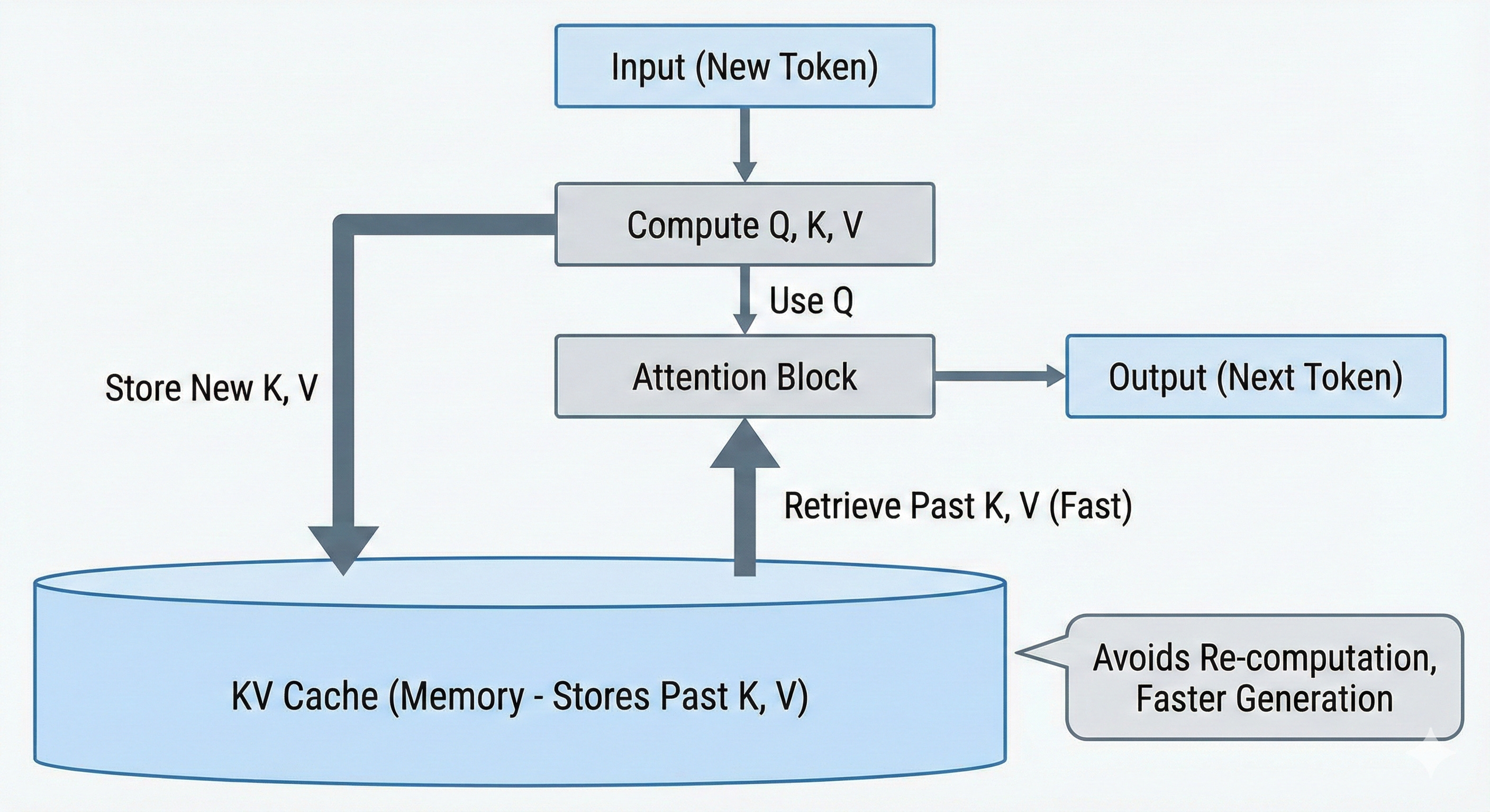
When generating token t_n, the model computes a Query vector q_n. It needs to compute the dot product of q_n with the Key vectors of all previous tokens k_1...k_n−1. If the model were to re-compute these Key vectors from the raw token inputs at every step, the computational complexity would be quadratic (O(n^2)), due to which real-time generation impossible.
To fix this, the Key and Value vectors for past tokens are computed once, as they are generated, and stored in GPU memory. This storage is the KV Cache. The KV Cache transforms the attention operation from a quadratic compute problem into a linear memory problem. Instead of recomputing, the model simply reads the history from VRAM.
If you are a visual learner checkout this video on KV cache for more intution.
The size of the KV cache is deterministic and can be calculated precisely. For a model with the following hyperparameters:
L_layers: Number of layers in the model.
d_model: Hidden dimension of the model.
H: Number of heads.
d_head: Dimension of each head (d_head = d_model / H).
B: Batch size (number of sequences).
S: Sequence length (number of tokens in context).
P: Precision in bytes (e.g., 2 for FP16, 4 for FP32).
In MHA, for every token in every sequence, we must store a Key vector and a Value vector for every head in every layer. The size of the Key cache for one layer is: B×S×H×dhead×P. Since H×dhead=dmodel, this simplifies to B×S×dmodel×P. We must store both Keys and Values, so we multiply by 2. We sum across all layers, multiplying by Llayers.
Size for MHA=2×B×S×L_layers×d_model×P
This formula reveals the linear scaling properties. The cache grows linearly with batch size and sequence length.
To illustrate the severity of this scaling, let us consider a practical example using the Llama 2 70B architecture (assuming MHA for demonstration, though the actual model uses GQA, which we will discuss later).
d_model=8192
L_layers=80
P=2 bytes (FP16)
B=32 (moderate batch)
S=4096 (standard context)
Size=2×32×4096×80×8192×2 bytes
Size≈343,597,383,680 bytes≈343 GB
Here on, we work on step by step motivating the need for Grouped Query Attention while understanding the GPU constraints we are working with.
The performance of an LLM on a GPU is governed by the interaction between the volume of data required and the speed at which that data can be processed. This interaction is captured by the Roofline Model, a performance model used to visualise the bounds of a computing system.
For a more in depth analysis, you can check out the previous blog on GPU Mental Models. It covers basic concepts like Arithmetic Intensity, Roofline Model, Compute vs Memory Tradeoffs, etc.
GPU Mental Models for Beginners

GPUs are all the rage these days, making them go brrr even more so. But what makes these highly parallel machines go that fast?
For this post’s discussion we only worry about two GPU bottlenecks explained below.
A. Compute Bound Operations
An operation is compute-bound when the arithmetic intensity is high enough that the system's throughput (amount of tokens it can process) is limited by the raw processing speed of the Tensor Cores. In a compute-bound scenario, the memory system delivers data to the cores faster than the cores can process it.
In the context of LLM inference, the Prefill Phase is predominantly compute-bound.
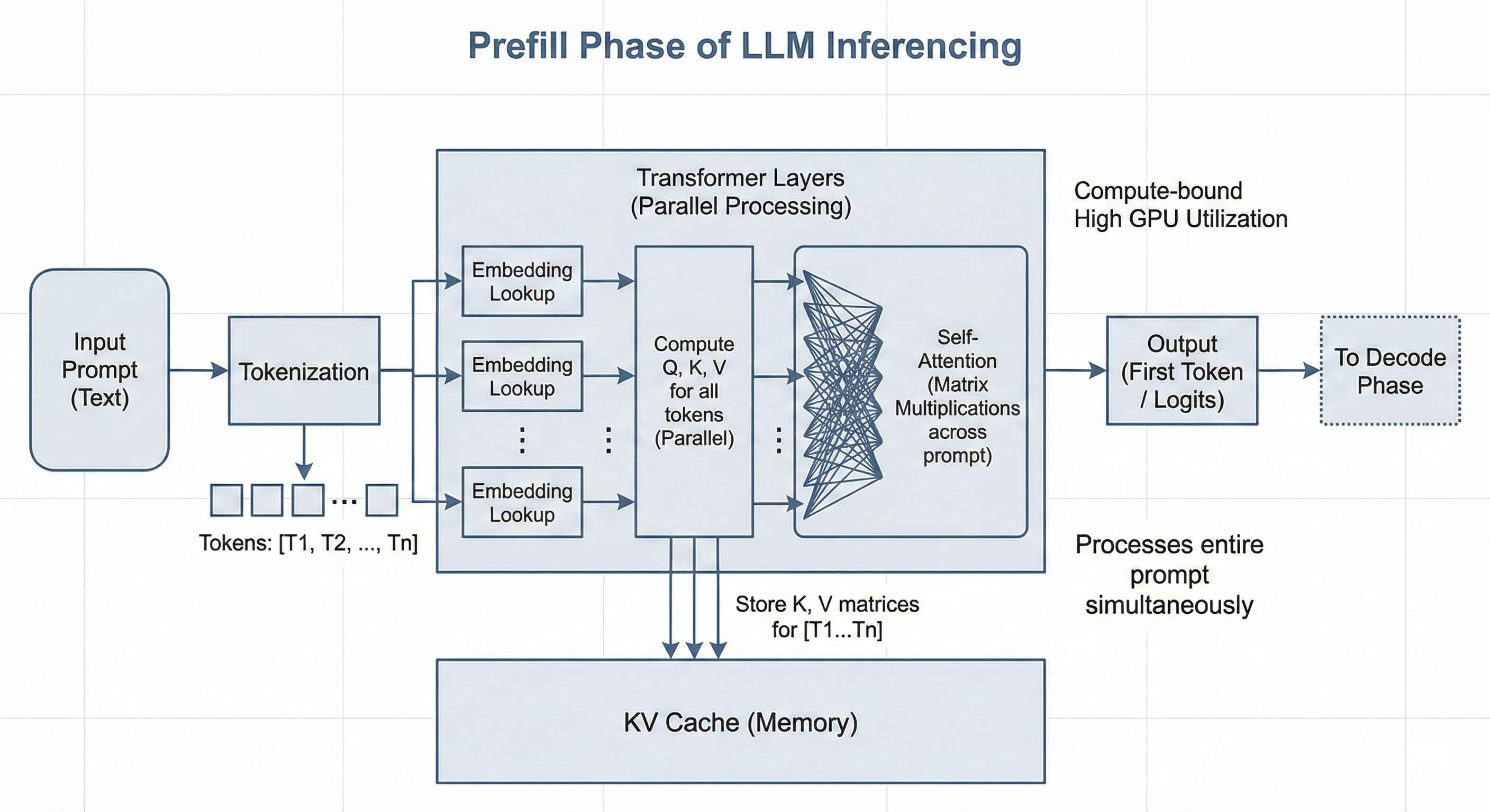
When a user submits a prompt, the model processes all input tokens in parallel. The Query (Q), Key (K), and Value (V) projections are matrix-matrix multiplications (GEMM), where the model weights are loaded once from High Bandwidth Memory (HBM) into the on-chip SRAM (Static Random Access Memory) and reused across the large batch of input tokens.
B. Memory Bandwidth Bound Operations
An operation is memory-bound when the arithmetic intensity is low, causing the compute cores to idle while waiting for data to arrive from HBM. The throughput in this regime is not determined by how fast the GPU can calculate, but by how fast it can move data.
This characterises the Decode Phase of LLM inference.
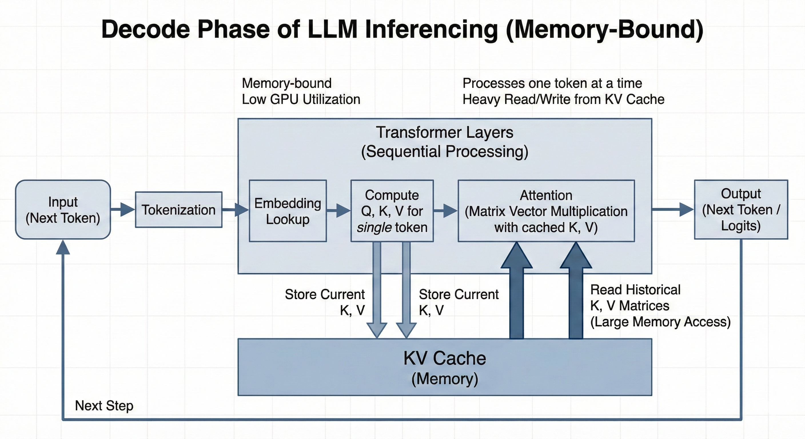
In autoregressive decoding, tokens are generated sequentially. To generate a single token, the model must perform a forward pass. This requires loading the entire set of model weights. Furthermore, in the attention layers, the model must interact with the history of the sequence. It does not recompute the entire history; instead, it loads the pre-computed Key and Value vectors from the KV Cache. Crucially, the matrix operations in this phase are matrix-vector multiplications (GEMV). The weight matrix is loaded, but it is applied to only a single token vector (or a small batch of tokens). The reuse of data is minimal.
Multi-Query Attention (MQA):“One Write-Head is All You Need”
The first major architectural response to the inference bandwidth crisis came in 2019 from Noam Shazeer at Google. In his paper “Fast Transformer Decoding: One Write-Head is All You Need” , Shazeer identified that the memory bandwidth overhead of loading the large Key and Value tensors was the primary bottleneck for incremental inference.
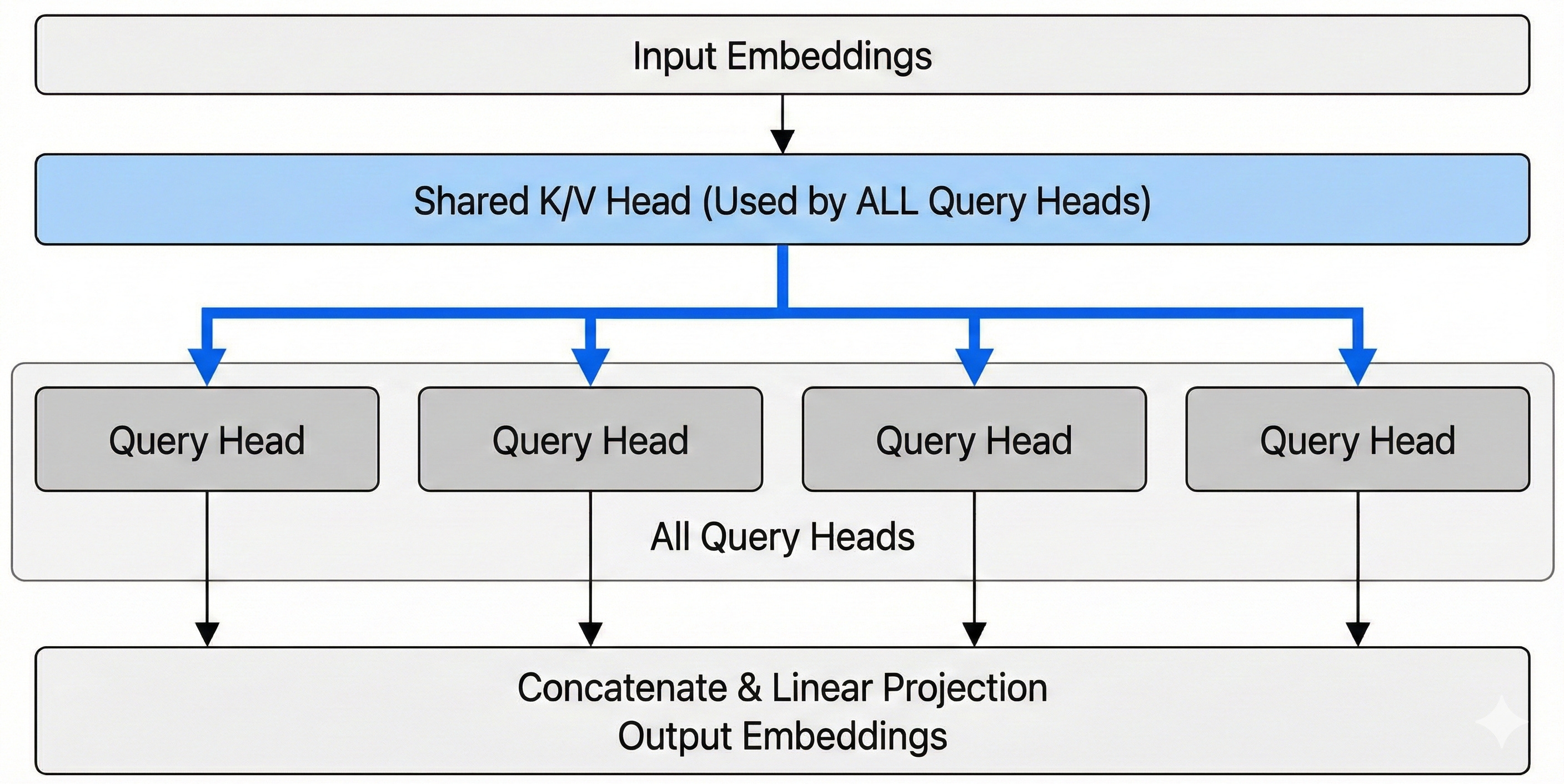
Shazeer proposed Multi-Query Attention (MQA). The core insight of MQA was that the redundancy in the Key and Value heads across different attention heads was largely unnecessary for model performance, yet incredibly expensive for memory bandwidth. While the Queries need to be diverse to ask different questions of the context, the Keys and Values (the representation of the context itself) could be shared.
MQA retains the multiple Query heads (H_q) of MHA but collapses the Key and Value heads into a single shared head for all queries.
Mathematically it boils down to:
This means that while each query head projects the input into a unique subspace, they all attend to the same underlying structure of the context (the single K and V).
The attention calculation changes from:
To below:
If we look at the theoretical performance gains:
The impact of MQA on the KV cache size is drastic. The reduction factor is equivalent to the number of heads (H).
Size for MQA= (2×B×S×L×D×P) / H
For a standard model with 32 or 64 heads, MQA reduces the KV cache size and the associated memory bandwidth requirement by a factor of 32x or 64x.
Revisiting our previous example of the 70B model with H=64:
MHA Cache: ~343 GB
MQA Cache: ~5.3 GB
Quality Trade-offs in MQA
Despite its massive efficiency gains, MQA was not immediately adopted universally in the years following its 2019 release. The primary barrier was the trade-off with model quality.
Model Quality: Compressing the key-value representation from H subspaces to 1 results in a loss of expressivity. The model struggles to capture nuanced semantic relationships (e.g., attending to syntactic structure vs. semantic meaning simultaneously).
Training Instability: It was also noted that training MQA models from scratch could be unstable compared to MHA. The drastic reduction in parameters in the projection layers (WK and WV) made optimisation more difficult.
This leads us directly to GQA!
Grouped-Query Attention
Grouped-Query Attention (GQA) generalizes the idea of MQA by introducing an intermediate number of key-value groups between 1 and H. Instead of sharing one K/V across all heads, we partition the heads into G groups, each group sharing its own set of key and value projections.
In other words, GQA uses multiple K,V heads (more than one as in MQA, but fewer than the number of query heads in MHA). If G = H, we recover standard MHA; if G = 1, we recover MQA. Typically, GQA implies some intermediate grouping (2, 4, 8, etc.), chosen as a hyperparameter.
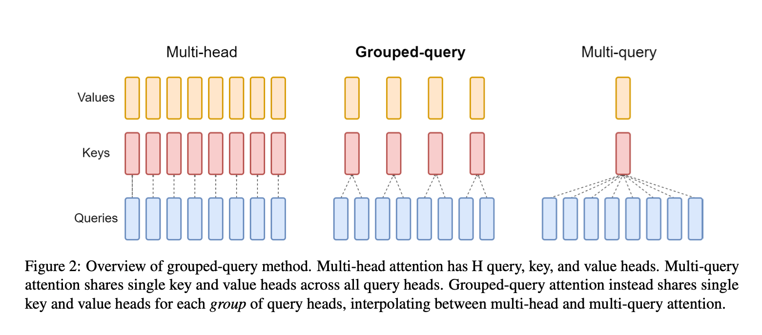
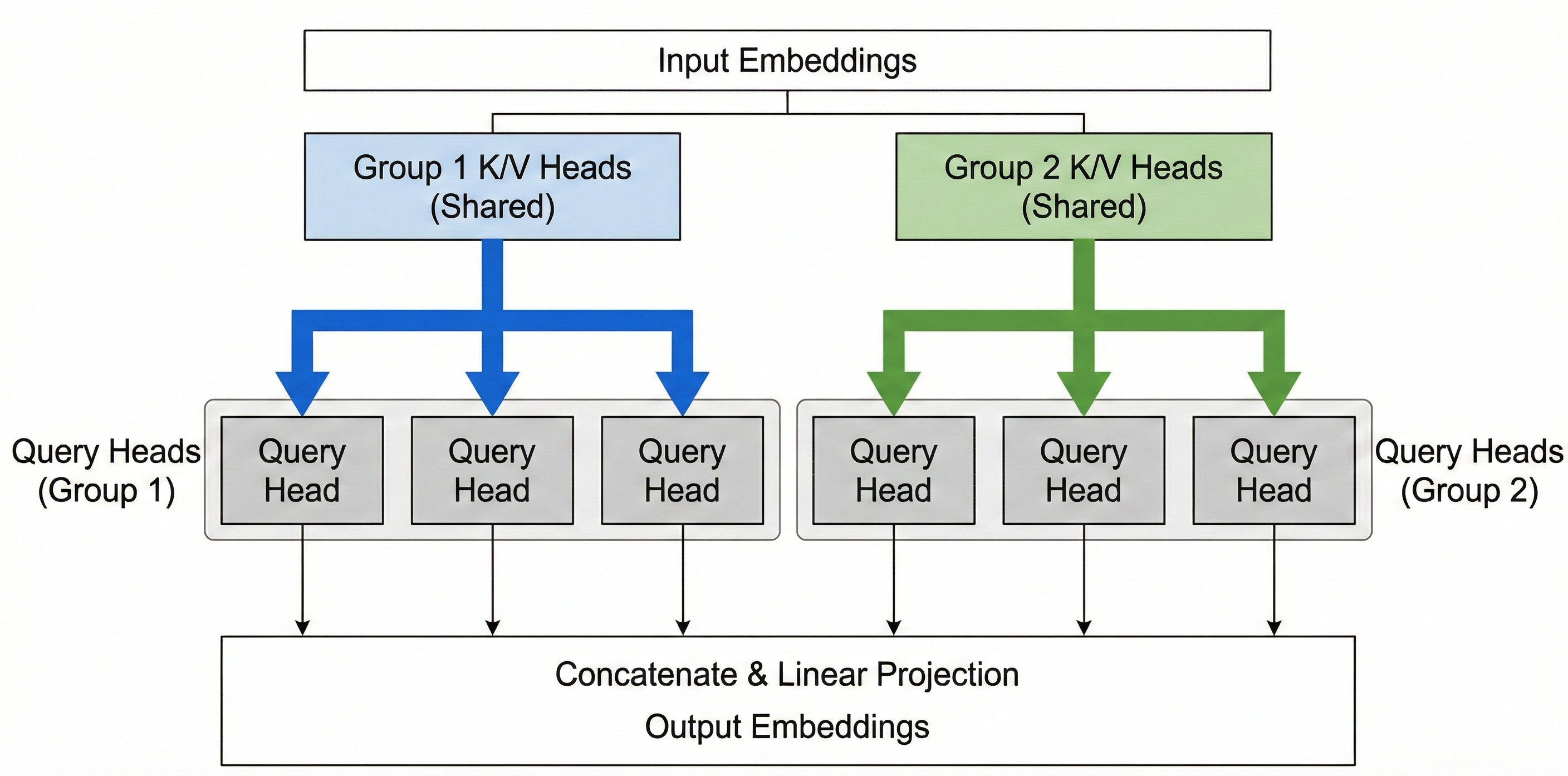
Suppose we have eight attention heads (H=8). With GQA we might decide to use, say, G=2 groups. Then we will have 2 distinct key heads (and 2 value heads) per layer. Perhaps heads 1–4 share key group 1, and heads 5–8 share key group 2. Each group has its own W_K and W_V projection matrices. At inference, each new token yields 2 key vectors and 2 value vectors (instead of 8 each in MHA). Each of those is then used by 4 query heads (whichever heads belong to that group).
In summary for GQA,
and following are the key advantages of using GQA
Memory savings: Like MQA, GQA leads to a smaller KV cache. Instead of H key/value vectors per token, we have G. This cuts KV memory by a factor of ~H/G.
For example, if a model has H=16 heads and we use G=4 KV groups, the KV cache becomes 4/16 = 25% of its original size (a 4× reduction). If G=2, that’s an 8× reduction; G=8 yields a 2× reduction, etc. These savings directly translate to lower memory capacity requirements and less bandwidth needed per token.
GQA therefore reduces memory overhead during inference similar to MQA (though not as extreme). It improves throughput by needing to retrieve and process fewer K,V pairs, mitigating the memory-bandwidth bottleneck. In practice, GQA is found to be nearly as fast as MQA for decoding, while using more memory than MQA but much less than MHA – it’s a tunable trade-off.
Model performance: Because GQA still uses multiple groups of keys/values, it retains more modeling capacity than single-head MQA. Ablation studies in the literature (e.g. the GQA paper and Meta’s LLaMA-2 paper) found that GQA can match the performance of full MHA on most tasks, despite the reduced parameters.
In other words, with a reasonable number of groups, accuracy drop is minimal – “nearly as accurate as MHA while being nearly as fast as MQA.” This makes it an attractive compromise.
Given these benefits, GQA was rapidly adopted in 2023 for large LLMs.
Here are the models which adopt GQA:
Meta’s LLaMA 2 (8 groups for 32 heads), LLaMA-3
Mistral 7B
IBM’s Granite 3B/13B
Implementation: RoPE Attention Module
Step1: Revisiting RoPE
Refer this blog for detailed intuition and implementation of Rotary Positional Embeddings

Step2: Handling Key-Value Compression (GQA)
To reduce memory pressure, GQA allows us to use fewer key-value heads (kv_heads) than query heads (num_heads). Each group of query heads shares a common set of keys and values. For this, we use a simple replication utility:
def repeat_kv(hidden_states, n_rep):
    batch, num_kv_heads, seq_len, head_dim = hidden_states.shape
    hidden_states = hidden_states[:, :, None, :, :].expand(batch, num_kv_heads, n_rep, seq_len, head_dim)
    return hidden_states.reshape(batch, num_kv_heads * n_rep, seq_len, head_dim)
Tidying it all together:
class RopeAttention(nn.Module):
    def __init__(self, config):
        super().__init__()
        self.hidden_size = config.hidden_size
        self.num_heads = config.num_heads
        self.kv_heads = config.kv_heads
        self.head_dim = self.hidden_size // self.num_heads
        self.rope_theta = 10000.0

        # Linear projections for query, key, value
        self.W_query = nn.Linear(self.hidden_size, self.num_heads * self.head_dim, bias=False)
        self.W_key   = nn.Linear(self.hidden_size, self.kv_heads  * self.head_dim, bias=False)
        self.W_value = nn.Linear(self.hidden_size, self.kv_heads  * self.head_dim, bias=False)

        self.W_output = nn.Linear(self.hidden_size, self.hidden_size, bias=False)

        self.rotary_emb = RotaryEmbedder(base=self.rope_theta, dim=self.head_dim)


    def forward(self, hidden_states: torch.Tensor, attention_mask=None):
        bsz, seqlen, _ = hidden_states.size()


        q = self.W_query(hidden_states).view(bsz, seqlen, self.num_heads, self.head_dim).transpose(1, 2)  # [B, h, T, d]
        k = self.W_key(hidden_states).view(bsz, seqlen, self.kv_heads, self.head_dim).transpose(1, 2)     # [B, kv, T, d]
        v = self.W_value(hidden_states).view(bsz, seqlen, self.kv_heads, self.head_dim).transpose(1, 2)   # [B, kv, T, d]


        cos, sin = self.rotary_emb(v)
        q, k = apply_rotary_pos_emb(q, k, cos, sin)


        kv_repeat = self.num_heads // self.kv_heads
        k = repeat_kv(k, kv_repeat)
        v = repeat_kv(v, kv_repeat)

        attn_scores = torch.matmul(q, k.transpose(2, 3)) / math.sqrt(self.head_dim)

        if attention_mask is not None:
            attn_scores += attention_mask


        attn_weights = nn.functional.softmax(attn_scores, dim=-1)

        context = torch.matmul(attn_weights, v)

        context = context.transpose(1, 2).contiguous().view(bsz, seqlen, -1)
        return self.W_output(context)
Conclusion
This implementation cleanly combines three ideas that define modern attention layers in LLMs:
Multi-head attention, for diverse feature subspaces.
Rotary embeddings, for relative positional awareness.
Grouped-query attention, for efficient inference memory use.
Together, they allow us to scale attention to long sequences and large models.
A very good and informative read.