
GPU Mental Models for Beginners
A gentle introduction to GPU architecture, memory hierarchies, and the mental models you need to optimise modern ML workloads.

GPUs are all the rage these days, making them go brrr even more so. But what makes these highly parallel machines go that fast?
The goal of this blog is to provide a beginner introduction to mental models for thinking about GPUs. How to think about the memory and compute of a GPU, their tradeoffs and everything in between. Without further ado, let’s jump in.

CPU vs GPU
To understand the hardware difference, we must first understand the optimisation goal.
There is a difference in key optimization goals for CPUs and GPUs:
CPUs are optimized for Latency
GPUs are optimised for Throughput
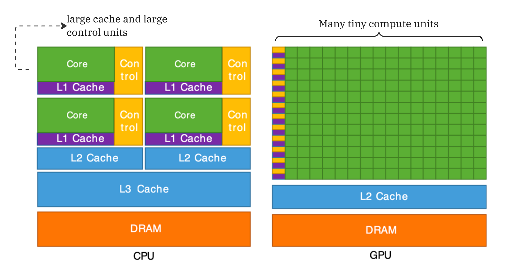
Structure of a CPU:
The Central Processing Unit (CPU) is designed to execute a single thread of instructions as quickly as possible. The key goal of a CPU is to execute sequential instructions at very fast speeds. For this, they have large control units and large caches. This is a direct consequence of optimizing for serial performance. A large amount of chip area is dedicated to control units and caches.
Large Control Units: This is because serial code is rife with conditional logic (if/else statements). To maintain high speeds, CPUs use branch prediction and speculative execution to keep the single thread running as fast as possible without stalling.
Large Caches: CPUs rely on large, multi-level caches (L1/L2/L3) to hide memory latency. Because the CPU aims to finish the current instruction immediately, it cannot afford to wait hundreds of cycles for data to arrive from RAM. It effectively hoards data close to the core to ensure the pipeline never stalls.
Structure of a GPU:
GPUs flip this logic. They operate on the SIMT Model, which stands for Single Instruction, Multiple Threads. They accept that individual threads will be slow but aim to maximize the total volume of computation per second.
Massive Parallelism: A GPU contains tons and tons of ALUs which are managed by smaller control units. Unlike CPUs with big control units, here a single Control Unit issues one instruction (e.g.,
tensor_add) to a group of 32 or 64 cores (often called a Warp, more on this later!) simultaneously.
Hence, summing it up:
“CPUs are optimised for latency (each thread finishes quickly), GPUs optimize for high throughput (total processed data)”
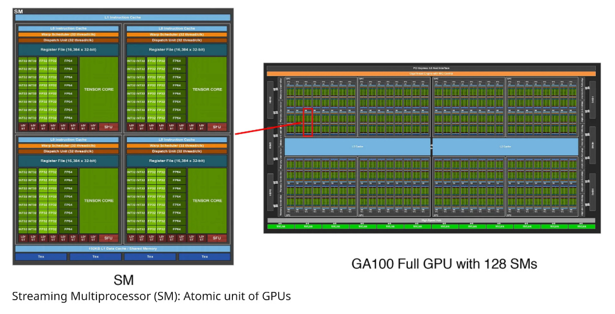
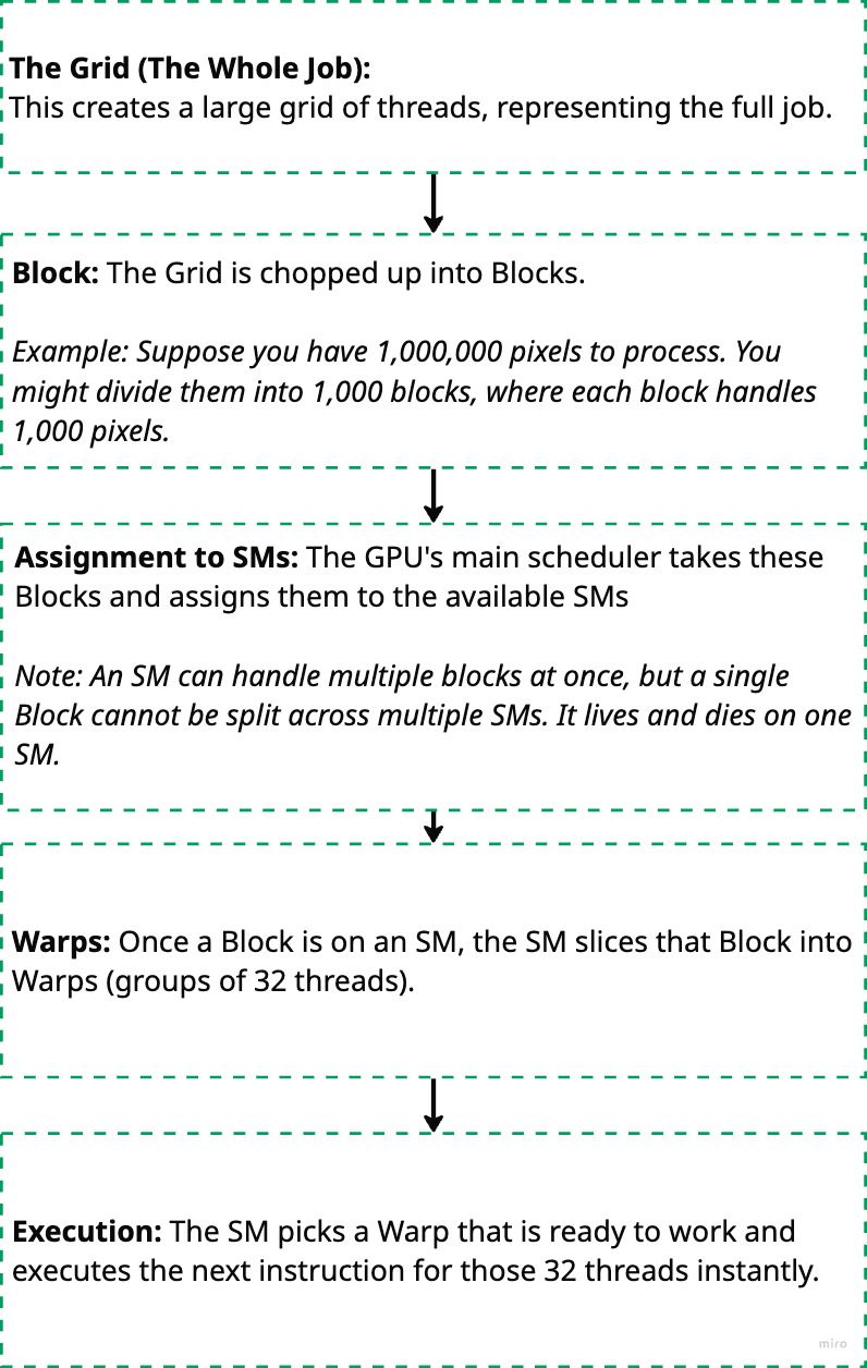
Anatomy of a GPU: SMs, Warps, Threads
A GPU has many atomic units called SMs (Streaming Multiprocessors). Each SM further contains many SPs (Streaming Processors) which execute threads in parallel. An SM has a bunch of control logic. SPs take the instruction and apply it to many pieces of data.
GPUs have many SMs (Streaming Multiprocessors) which are essentially the atomic units. Even when we code in Triton, we are operating at the SM level. Each SM independently executes “blocks” of jobs.
Each SM further contains many SPs (Streaming Processors) that can execute “threads” in parallel.
Each SM has a bunch of control logic-it can do, for example, branching.
Execution Model of a GPU
Let’s start with threads:
Thread: A Thread is the smallest unit of execution. A thread runs your code. It has its own small workspace (registers) and knows “who” it is (its ID).
Warps: A set of 32 threads that execute the same instruction at the same time. This is where the SIMT, “Single Instruction Multiple Threads” model comes in.
Blocks: Blocks are groups of threads. Each block runs on an SM with its own shared memory. Threads in the same Block can talk to each other using a fast, shared memory cache (Shared Memory).
SM: Streaming Multiprocessor. This is the actual hardware on the GPU. Each SM may have its own scheduler, registers, and cache.
Grid: The entire problem (e.g., “Process this 1080p image”).
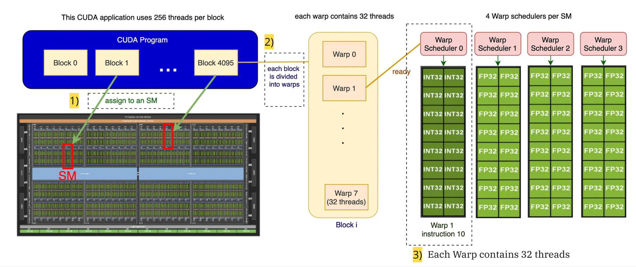
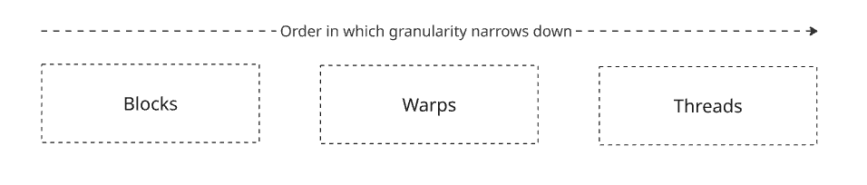
When you run code on a GPU, work is organized into several layers, from the high-level program down to the hardware execution. Here’s the typical order:
GPU (Hardware) contains many SMs → SM executes one or more Blocks → Block contains many Warps → Warp contains 32 Threads.
Below diagram summarises the logical flow of execution:
Memory Model of a GPU
Understanding GPU memory is just as critical as understanding compute. While compute measures how much work we can do (in floating point operations), memory structure and bandwidth determines how fast we can read and write the data needed for those operations.
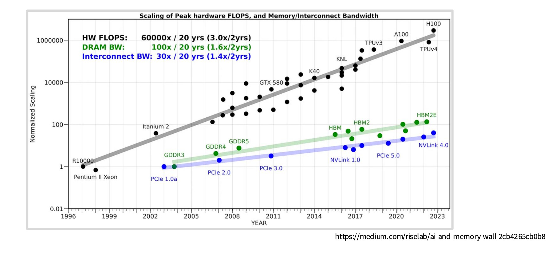
This distinction matters because most modern LLM workloads are memory bound, not compute bound. In other words, the GPU cores spend more time waiting for data to arrive than actually performing calculations.
The core problem: compute capability (number of floating point operations per second) has been scaling much faster than memory bandwidth. This growing gap means memory increasingly becomes the bottleneck, even as our GPUs get more powerful.
Having a rough understanding of the physical structure of the GPU helps in this case. When operating at such fast speeds, physical proximity to where the computation happens becomes more important than we expect.
In this section we are going to talk about a lot of complicated memory hierarchies, both independently and in their relation of proximity with the SMs.
But before we jump in, we look at the two hardware technologies used to build memory:
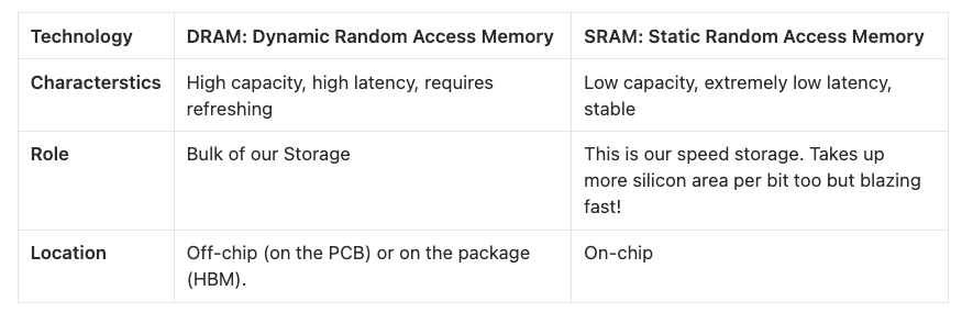
SRAM is much more expensive but 8x faster than DRAM.
The Memory Hierarchy (Farthest to Closest)
We will walk from the massive storage outside the chip into the heart of the execution units.
A. Global Memory (The VRAM)
Technology: DRAM
Scope: Accessible by all SMs and the CPU
Role: This is the “80GB” listed on an A100 spec sheet. It holds your model weights, optimizer states, and entire datasets.
Latency: Very High (~200–400+ cycles)
B. L2 Cache
Technology: SRAM
Scope: Shared across all SMs on the GPU
Role: The middleman. It sits between the slow Global Memory and the fast SMs. It caches data fetched from Global Memory so that if multiple SMs need the same data (common in convolution or attention mechanisms), they don’t all have to hit the slow DRAM.
Latency: Medium (~200 cycles)
Physical Location: On-chip, connected to the memory controllers
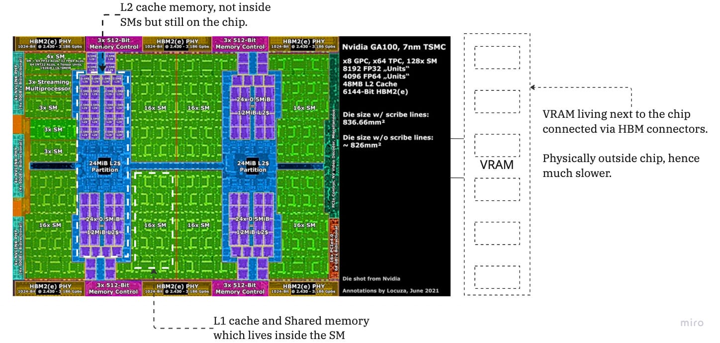
C. The SM Internal Memory (L1 & Shared Memory)
This is where the magic happens. Inside each Streaming Multiprocessor (SM) is a configurable block of fast SRAM. In modern architectures (like Ampere/Hopper), this block is physically unified but logically partitioned into two distinct uses:
1. L1 Cache (Hardware Managed)
Role: Standard caching. You generally do not control this. The hardware automatically stores frequently accessed Global/L2 data here.
2. Shared Memory (Software Managed / Programmable Cache)
Role: This is the most critical concept for kernel optimization. It is a manual cache that you (or the kernel writer) explicitly control.
Mechanism: You load a chunk of data (e.g., a tile of two matrices) from Global Memory into Shared Memory once. Then, the threads in that SM (the Warp) can reuse that data hundreds of times at SRAM speeds without touching Global Memory again.
Latency: Extremely Low (~20–30 cycles)
Why it matters: This is the primary mechanism for Tiling. Without Shared Memory, matrix multiplication would be impossibly slow because every operation would require fetching data from DRAM.
The proximity mental model for ML:
The closer the memory to the SM, the faster it is. L1 and shared memory is inside the SM. L2 cache is on die, and global memory are the memory chips next to the GPU.
The Roofline Model: Are You Compute Bound or Memory Bound?
The Roofline Model is a visual performance model used to determine the limiting factor of a specific process (say, a Kernel) running on a specific GPU. It plots Performance (GFLOPS) against Arithmetic Intensity (FLOPs/Byte).
Arithmetic Intensity:
This is the X-axis of the model. It measures how much work you do per byte of data fetched from global memory.
Low Intensity: Element-wise operations (e.g., ReLU, adding two vectors). You do 1 math operation for every 4 bytes read.
High Intensity: Dense Matrix Multiplication (GEMM). You load a tile of data and reuse it for many multiply-accumulate operations.
The model reveals two distinct performance ceilings:
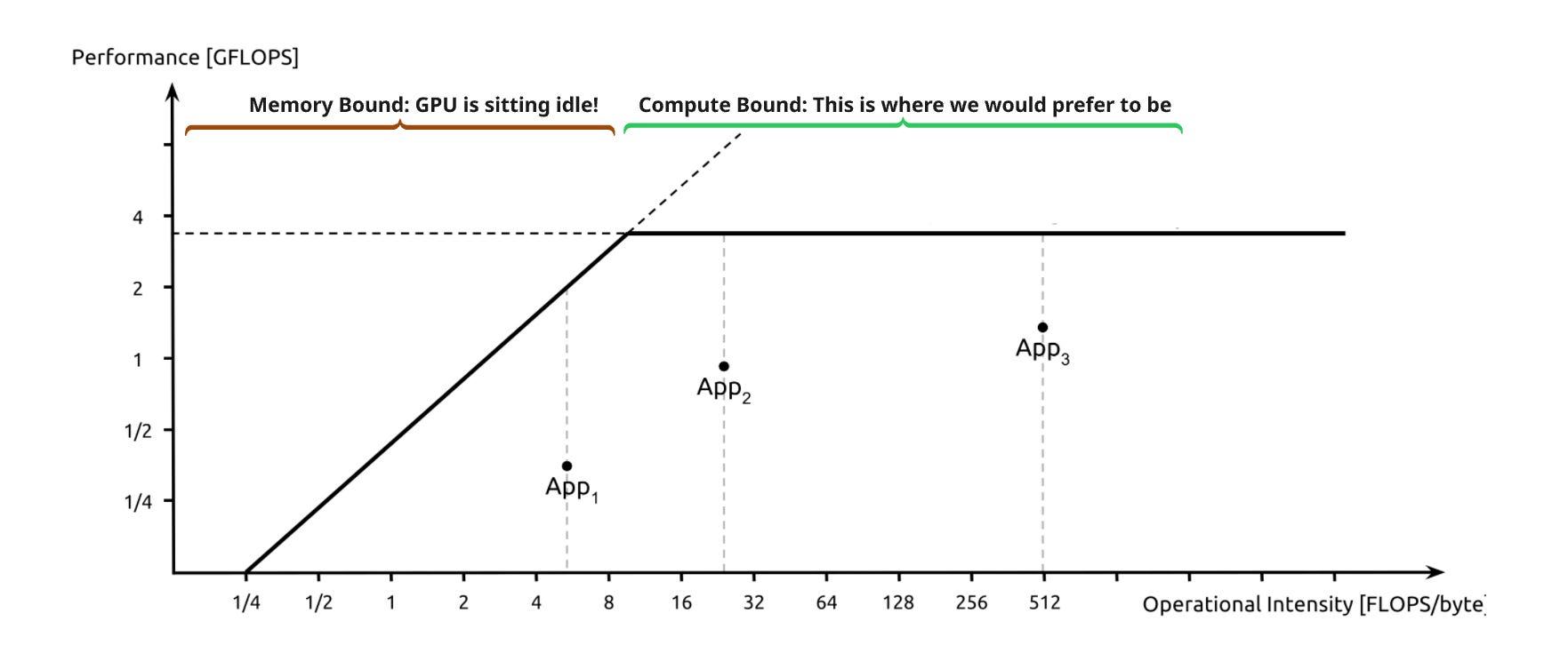
A. The Slanted Roof (Memory Bound)
Scenario: Your Arithmetic Intensity is low.
The Bottleneck: The GPU cores are starving. They process data faster than the memory bus can deliver it.
The Implication: Optimization efforts focused on faster math (e.g., using Tensor Cores) will have zero impact. To speed this up, you must increase memory bandwidth usage or increase arithmetic intensity (e.g., via kernel fusion).
B. The Flat Roof (Compute Bound)
Scenario: Your Arithmetic Intensity is high enough to saturate the compute units.
The Bottleneck: The memory system is delivering data fast enough, but the ALUs are fully utilized.
The Implication: You have hit the theoretical peak GFLOPS of the device. To speed this up, you must reduce the total number of operations or move to a faster GPU.
A simpler way of looking at this is: we want to make as few slow global memory accesses as possible and be fully utilizing our GPU cores without waiting for data.
So how is all this theoretical information used in the real world?
1. LLM Architecture: GQA vs. MQA vs. MHA
This is fundamentally a Memory Bandwidth optimization. In autoregressive decoding, fetching the Key-Value (KV) cache from Global Memory (DRAM) is the bottleneck, not the compute.
MHA (Multi-Head Attention): Requires loading a massive unique KV cache for every query head, often hitting the memory bandwidth “roof.”
MQA (Multi-Query Attention) & GQA (Grouped-Query Attention): These drastically reduce the size of the KV cache (by sharing keys/values across heads). This reduces the total bytes transferred per token generation, moving the operation away from the memory-bound limit and allowing higher batch sizes.
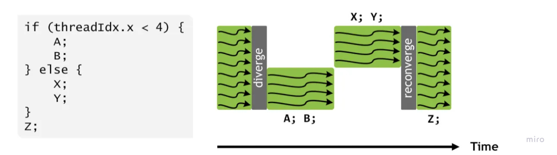
2. Control Divergence
This maps directly to the SIMT (Single Instruction, Multiple Threads) execution model.
The Cost: When you write conditional logic (
if thread_id < x...) inside a kernel, you fracture the Warp. The hardware must serialize execution, running theifpath while theelsethreads sleep, and then vice versa.The Fix: We design kernels to minimize branching or use “predicated execution” (masking) to keep all 32 threads in a Warp active and synchronized, maximizing instruction throughput.

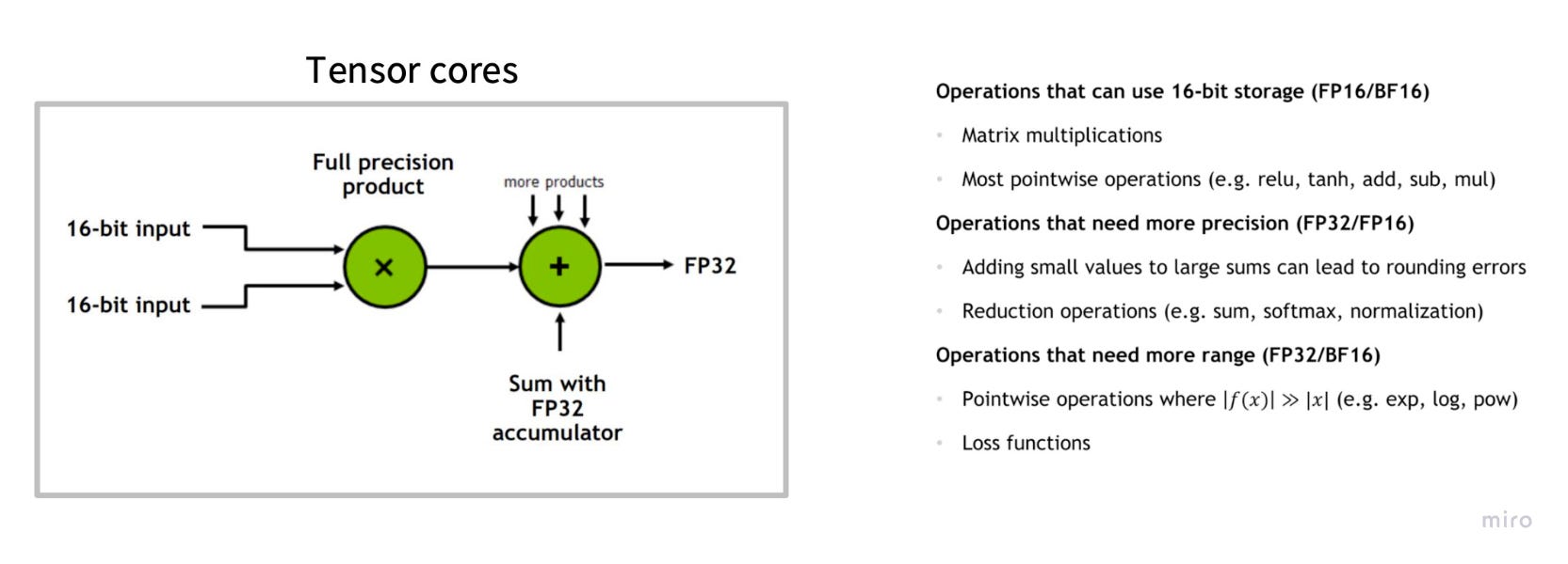
3. Low Precision Computation (Quantization)
This leverages the Throughput vs. Latency trade-off and the specialized Tensor Cores.
Bandwidth: Moving FP16 (2 bytes) instead of FP32 (4 bytes) instantly doubles your effective memory bandwidth. FP8 quadruples it.
Compute: Modern GPUs (H100/A100) have specialized Tensor Cores that execute low-precision matrix multiplies (A × B + C) at 2x–4x the speed of standard FP32 cores. We trade a tiny amount of numerical precision for massive gains in arithmetic intensity and raw FLOPS.
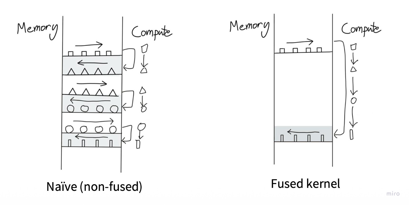
4. Operator Fusion
This is a Roofline Model optimization to fix Arithmetic Intensity.
The Problem: Running
Load → Add → Storefollowed byLoad → ReLU → Storewastes time moving data back and forth to slow Global Memory (DRAM).The Fix: “Fuse” these operations into a single kernel (
Load → Add → ReLU → Store). This keeps the data in fast Registers or L1 Cache between the addition and the activation, drastically increasing the ratio of math-to-memory operations.
5. Tiling
Tiling is another critical optimization where large matrices are broken into smaller tiles that fit in faster memory (shared memory/cache). This reduces global memory access and improves performance. Modern CUDA libraries like cuBLAS heavily use tiling for matrix operations. [I’ll explore this in detail in a future post.]
Conclusion
If you’re reading this, you probably care about making something faster, a model, a kernel, an entire training pipeline. And now you have the mental models to actually know where to look.
The beautiful thing about understanding GPU hardware is that it demystifies so much of what seems like black magic. Why does Flash Attention work? It’s exploiting shared memory to maximize arithmetic intensity. Why is batch size so critical for inference? You’re amortizing the fixed cost of loading weights from DRAM. Why does everyone freak out about memory bandwidth in the H100 specs? Because it’s the actual bottleneck for most real workloads.
The key insight? Data movement, not computation, is the hurdle.
Now you know what makes these highly parallel machines so special. Go make yours go faster.